
Using Statistics to Justify New Equipment: Establishing Normal Data Distribution Helps Calculate Possible Savings
Using Statistics to Justify New Equipment: Establishing Normal Data Distribution Helps Calculate Possible Savings
ISE Magazine February 2021 Volume: 53 Number: 2
By Merwan Mehta
https://www.iise.org/iemagazine/2021-02/html/mehta/mehta.html
Various statistical packages are available to conduct analysis and learn insights that would not be evident simply by looking at data. However, a lot can be achieved by using basic statistics in Excel.
To illustrate, let us say you have a ma-chine that is filling cereal boxes. The tar-get for the weight of the cereal in the box is 1,000 grams. We want to ensure we do not send a box with less than a full kilo-gram of cereal, and due to limitations of the machine, we have decided to allow a plus tolerance of 50 grams. Hence, the operating specification for the machine is 1,025 grams +/- 25 grams.
Say each cereal box filling machine produces 5,000 boxes per day and the cost of goods for the cereal is $1.50 per box or $1.50/1,000 = $0.0015 per gram. A new vendor says her machine can control the variation in the filling machine twice as effectively. We would like to evaluate this claim and estimate how much savings can result from the new machine.
Evaluating the current output
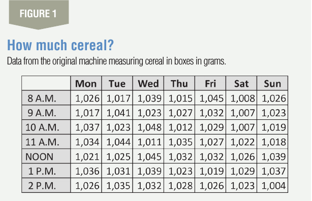
To begin the analysis, a good first place would be to first look at how well the present machine is performing. Figure 1 shows data for seven days of continuous running.
Before applying the properties of the normal distribution to the data, it is necessary to check whether the machine is producing normal data. One way to do this is to plot a histogram with an appropriate bin size in Excel and see if the resulting graph is a bell-shaped curve. In a normal distribution, most data points are concentrated near the average and show an equal tapering on both sides forming a bell-shaped curve. To do this, we use the histogram function in Excel under Data and Data Analysis. When the function is activated, select the data array with all data structured as a column and a bin array. We have created the bin array with a bin size of 5 grams, which should give us a histogram with between 10 to 15 bins.
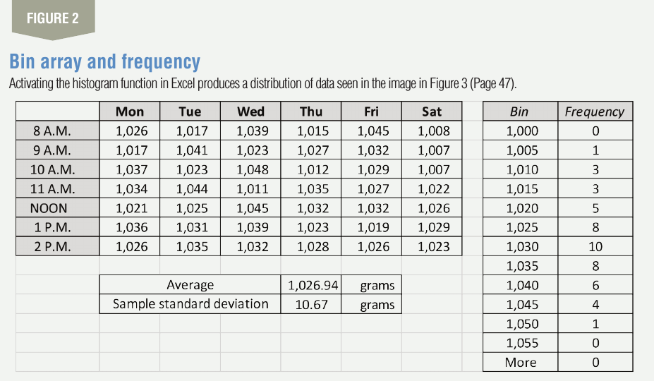
The bin array should begin with the minimum reading in the data set and end at the maximum reading or a little beyond. The creation of the bin array and the resulting frequency column after activating the histogram function is shown in Figure 2. Based on this data, using Excel we can calculate the mean for all 49 data points to be 1026.94 grams and the standard deviation (SD) to be 10.67 grams. We use the “average” and “STDEV.S” function in Excel to do this.
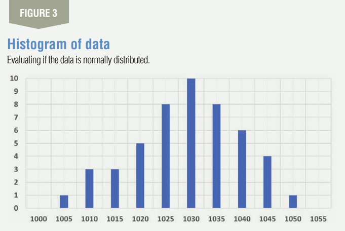
The frequency column is now plot-ted as a column chart to give you the histogram as shown in Figure 3. As can be seen from the histogram, that it is a normal-looking distribution, and hence it is OK for us to proceed further.
Using Excel, we can also use the correlation function under Data and Data Analysis to see if the data are normal or not by letting Excel calculate the R-square value if we are uncomfortable to conclude the data is normal by simply looking at the histogram. If the R-square value in the correlation function is greater than 0.8, we can safely conclude that the data are normal and proceed further.
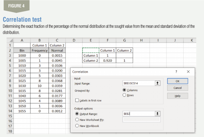
To do this, we create a column titled “normal” beside the frequency column as shown in Figure 4 and fill it with data using the formula for NORM.DIST. This function gives you the exact fraction of the percentage of the normal distribution at the sought value if you put in the mean and the standard deviation of the distribution. For example, the formula that gets 0.0015 under Column 2 is NORM.DIST (X, Mean, Stdev, False) or NORM.DIST (1,000, 1026.94, 10.67, False).
Here we are finding the percentage of the distribution in the 1,000 bin. Another example, 0.0045 or 0.45% of the cereal boxes have an average weight of 1,005 grams, and so on. Once the Column 2 for the normal data is created, run the correlation function from Data and Data Analysis by putting in the input range and the output range as shown in Figure 4. The correlation coefficient comes out to be 0.92 and, since it is above 0.8, we can safely assume the data to be normal.
For the data, we can also calculate how much of the product will be out-side the specification limits by using this formula: % of product below LSL = NORM.DIST (LSL, mean of data, SD of data, true), and above USL = 1 – NORM.DIST (USL, mean of data, SD of data, true). Hence, the % below LSL = NORM.DIST (1,000, 1,026.94, 10.67, True) = 0.58%, and USL = 1 – NORM.DIST (1,050, 1,026.94, 10.67, True) = 1.53%. We conclude that the company is shipping 0.58% of cereal boxes with less a kilogram of cereal and 1.53% of the boxes with more than 1,050 grams of cereal.
Based on the empirical rule of statistics we know that 99.73%, which is practically the entire distribution of data, will lie between mean plus and minus 3 times the standard deviation. These two limits are generally referred to as the lower control limit (LCL) and the upper control limit (UCL). Hence, for our process, LCL = mean – 3 x SD = 1,026.94 + (3 x 10.67) = 994.93 and UCL = mean + 3 x SD = 1,026.94 + (3 x 10.67) = 1,058.94.
At this point, we can calculate the process loss. As the mean of the sample is 26.94 grams (1,026.94 – 1,000) above the specification of 1,000 grams, each ma-chine is costing 26.94 x 5,000 x 0.0015 = $202.05 per day in excess cereal being given away.
Comparing old to the new
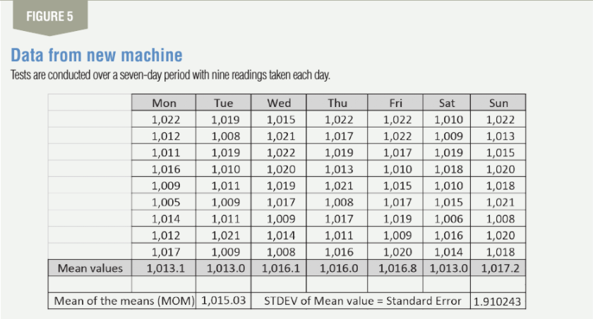
Now let us compare this data to the new equipment manufacturer who claims that their machine has half the variation of the present machine. Conducting tests on the machine, the data shown in Figure 5 is collected over a seven-day period. Nine readings are taken each day; the sample size is nine. We choose a sample size which has a complete root for ease of further calculations.
Applying the central limit theorem (CLT) of statistics, we can now estimate the standard deviation for the new population. CLT tells us that the distribution of the means of samples will be normal if the distribution from where the samples are drawn is normal, and the sample size is at least five. If we cannot assume that the distribution from where the samples are drawn is normal, we need to at least use a sample size of 25. The standard deviation of the mean values drawn from the new population is called the standard error (SE), and the CLT allows us to estimate the standard deviation of the population using this formula: SD of the population = √(Sample size) x SE.
For our data, the SD of the means drawn from the sample or the SE = 1.91. Using this, the SD of the population from the new machine = √(9) x 1.91 = 5.73 grams. The old machine had a SD of 10.67, hence the claim of the new ma-chine vendor that the SD of its machine is half that of the old machine is not completely true as it comes out to be 0.54 (5.73 / 10.67) and not 0.5. The CLT also helps us estimate the mean for the population, which is calculated by taking the means of all the means (MOM), which comes out to be 1,015.03 grams.
We can now calculate the LCL and the UCL for the new machine by using LCL = mean – 3 x SD = 1,015.03 + (3 x 5.73) = 997.84 and UCL = mean + 3 x SD = 1015.03 + (3 x 5.73) = 1,032.22.
For the new machine, we can now calculate how much of the product will be outside the specification limits by previously shown formula. Hence, the % below LSL = NORM.DIST (1,000, 1,015.03, 5.73, true) = 0.44%, and USL = 1 – NORM.DIST (1,050, 1,015.03, 5.73, true) = 0.00%. We see that with the new machine, the company will be ship-ping fewer boxes that are under the 1,000 gram weight and no cereal boxes greater than 1,050 grams of cereal.
As calculated above, the mean of means (MOM) for the new machine is 1,015.03, which is the best estimate for the mean of the new machine. We can now calculate the p-value for the hypothesis test of comparing the means of the old and the new machines.
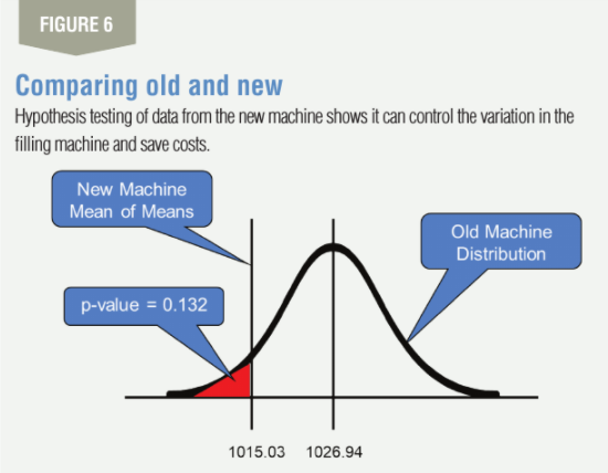
The original distribution has a mean of 1,026.94 and a SD of 10.67. We would now want to know whether the MOM can be assumed to be from the old population or not.
To get the p-value for this, we use p-value = NORM.DIST (1,015.03, 1,026.94, 10.67, true) = 0.132. This tells us that there is only a 13.2% probability that the MOM that we got of 1,015.03 is because of chance. If we use a confidence level of 95%, we can say that the two means are the same as the p-value that we calculated of 0.132 is greater than the level of significance of 0.05, which is 100% minus the confidence level. The hypothesis testing is shown graphically in Figure 6.
We can now also calculate how much it costs for the extra cereal being given away. As the MOM is 15.03 grams (1,015.03 – 1,000) above the specification of 1,000 grams, each new machine is costing 15.03 x 5,000 x 0.0015 = $112.73 per day in excess cereal being given away. Hence, this is a saving of $202.05 – $112.73 = $89.32 per machine per day. This might be enough to finance a good part of the new machine, and thus going in for the new machine might be a good decision.
Engineers and technologists are taught a lot of statistics, but for evaluating equipment, basic statistical properties of the normal distribution can suffice. Using the empirical rule of statistics and the central limit theorem, we can also conduct a test of hypothesis. The key is to ensure first that the data is normal for us to proceed to applying the properties of the normal distribution.
Without using the CLT, the equipment manufacturer was claiming her equipment had half the variation of the old equipment might use the entire 63 readings, which taken as one sample will give us a mean of 1,015.03 grams and a standard deviation of 4.88, which she can claim is less than half (4.88 / 10.67 = 0.46) the original variation.
However, using the CLT, it gives us the true standard deviation of the new machine as 5.73 grams. Using the NORM.DIST function to calculate the area under the normal distribution also allows us estimate what percentage of the output will be outside the specification levels.
Comments :